AI-1 — the gating model

AI-1 is Cytogence’s own gating model. It is not a large language model and it is not the copilot.

It runs entirely on your machine. No account, no API key, no network. A run takes a few minutes on a million-event file, longer on a slower computer — and the app tells you how long to expect on yours (below).

Using it requires a license; the 30-day trial includes it.

Where to start it

Two places, both running the same model on the same file:

• The AI-Guided Gating panel — click AI in the gating toolbar, then Identify populations with the Cytogence model. This is the dedicated panel, where the competence report has the most room.
• The copilot — opening the copilot with a file loaded offers to run the gating model first (Run it / Not now), and a Gating model control stays in its header for the rest of the conversation.

The second exists because the first was hard to find. The copilot is where people go when they want help, and it had no way of telling you that the better tool for identifying populations was sitting behind a different button.

How long it takes, and why it uses the CPU

AI-1 runs on the CPU, by design. It is implemented directly in the application, with no machine-learning runtime, and spreads its work across your processor’s cores. It does not use the GPU — also when a local language model is using it — so high CPU use for a few minutes on a large file is expected, not a fault.

While it runs, you see the elapsed time against an estimate:

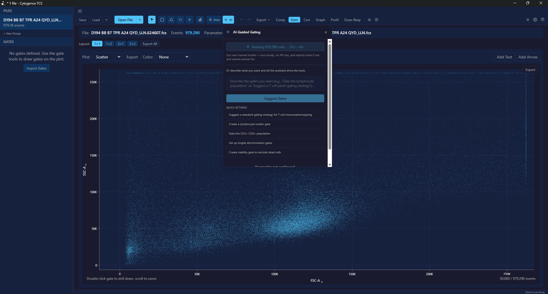
• In the AI-Guided Gating panel, the button shows Reading … cells… with a counter such as 42s / ~300s. If the run passes the estimate, the counter says longer than expected — the model is still working, not stuck.
• In the copilot, a Cytogence gating model — running card shows, for example, 42s elapsed · about 5 minutes on this machine. If the run passes the estimate, the card says Taking longer than estimated — still working.

The estimate is learned on your machine. Before your first completed run it starts from a conservative rate, and the copilot marks it (estimated). Each completed run on a file of at least 50,000 events then updates it, weighted toward the most recent run, so the estimate follows your hardware rather than ours. It is also deliberately pessimistic — it assumes your machine is about 25% slower than it measured — so a normal run finishes ahead of the number on screen.

This used to be the opposite, and the reason is worth knowing if you are reading an older copy of these docs. Before v0.1.9 the estimate was a fixed constant. It was measured honestly when it was written, and then the model grew and nothing updated the number. It went on promising about 48 seconds for a run that had come to take minutes.

Before 0.2.2, on a computer without graphics acceleration — a virtual machine, a Remote Desktop session, or a disabled graphics driver — an open plot itself used a lot of CPU and slowed AI-1 considerably. Plots now redraw only when something on them changes; if you run Cytogence FCS that way, update.

When a result is reused

Recent results are kept in memory, per file, for the rest of the session; nothing is written to disk.

• When the copilot needs AI-1 to build a gating hierarchy for a file it has already run on in this session, it reuses that result instead of running the model again — so a second request on the same file does not wait.
• When you start a run yourself — the panel button, Run it, or the Gating model control — the model runs again from the start, with a fresh progress counter.

A file that has changed on disk is never served an old result.

What it identifies

Nine populations, on human samples. These describe the model shipping today — the figures are tied to the trained model, which changes on its own schedule, rather than to the application version:

Population	Precision	Recall	F1	F1 range across splits
B cells	0.938	0.950	0.944	0.933–0.953
NK cells	0.925	0.960	0.942	0.914–0.960
Lymphocytes	0.919	0.924	0.921	0.900–0.942
NK-T cells	0.929	0.903	0.916	0.896–0.931
CD3⁺ T cells	0.890	0.899	0.893	0.838–0.924
CD8⁺ T cells	0.859	0.924	0.890	0.859–0.906
Live lymphocytes	0.866	0.909	0.885	0.764–0.929
CD4⁺ T cells	0.824	0.873	0.846	0.806–0.889
Monocytes	0.746	0.826	0.782	0.753–0.807

Eight of these are reported as populations; CD3 is the stage the CD4 and CD8 chains pass through, and appears in your gate tree as their parent.

How these were measured, because the protocol is the claim: the mean over eight independent train/validation/test partitions, split 60/20/20 by sample so a sample never trains one population and tests another; thresholds chosen on validation, every reported number taken from the untouched test split; each population scored in the configuration the product actually ships, over all events including its parent chain rather than inside a parent an expert already drew. Ground truth is expert FlowJo gating on human peripheral blood and PBMC.

That “shipped configuration” clause is the one that matters. It is easy to publish a better-looking number by scoring a population inside the expert’s own parent gate — and that describes a product nobody ships. These are end-to-end numbers.

The range matters as much as the mean. Live lymphocytes runs 0.764–0.929 across splits because only 85 samples carry that label; it is the least-supported figure here. A single split would have let us quote the top of that range and call it the result.

What changed with this model

Every population improved over the previous encoder and none regressed. The largest gain is Monocytes (+0.043), which had been sitting on the bar we require and now has real margin.

The T-cell branch also became a single decision rather than three independent ones, so CD4 and CD8 now sum exactly to their CD3 parent instead of approximately nesting. If you previously saw subsets that didn’t quite add up, that’s why.

Your samples will differ from these cohorts

These come from public human immunology studies. Your panel, instrument and staining are not those cohorts, which is exactly why the model reports its own competence per population per file rather than assuming these figures transfer. See the competence report.

That is the whole list. It is deliberately short, and published rather than implied, because a model whose scope you cannot state is a model you cannot check.

If you used v0.1.1: “Live cells” is now “Live lymphocytes”

The population previously labelled Live cells reported roughly 95% on a typical sample. That number was wrong for the label — the gate was learned from expert labels that mean live cells within lymphocytes, not whole-tube viability, and reporting it as whole-tube viability overstated it several-fold.

It now ships as Live lymphocytes, nested under Lymphocytes. The number is smaller because it is now measuring what it says it measures — how much smaller depends on your sample, since it is a fraction of the lymphocytes present. Agreement with expert gating went from 0.56 to 0.885 in the process.

If you have v0.1.1 figures in a notebook, this is why they changed.

What it refuses to identify, and why that is the point

AI-1 is built to abstain and say why rather than guess.

Four populations are deliberately withheld, each for a stated reason:

Withheld	Why
Dendritic cells	Blocked on data. The markers that actually define DC subsets aren’t available in the training material we can use.
Monocyte subsets	Classical monocytes scored worse than predicting everything positive. A gate that adds nothing is worse than no gate, because it looks like information.
Singlets	Same reason, within its parent.
T cells (as a single population)	It would not nest consistently with CD4-T and CD8-T, so the tree would stop adding up.

Every population must clear a fixed precision and recall bar before it is offered. Populations that clear it are gated; populations that do not are named as gaps. We would rather ship a short list you can trust than a long one you have to check.

The bar is not cosmetic: monocytes spent a release on it, clearing on only three splits out of four, and were held back until they cleared on all of them.

Anything outside the list is out of repertoire, and the model says so instead of producing a confident answer.

Why human samples only

This is the result that shaped the whole design.

On mouse data, the model’s ranking held up well — it still separated CD3⁺ from CD3⁻ cells about as cleanly as it does in human samples. But its calibration collapsed completely: at the thresholds learned from human data, the resulting gates were worthless.

A model that reported only “confidence” would have looked fine and been useless. That is why competence here is not a single number.

The abstention is measured, not asserted

We ran the shipped model, with zero tuning, against a human study it had never seen — a 2013-era Treg study on different instruments with different staining.

Every sample landed far outside the distribution the model was trained on, and the product abstained and withheld the figures on all of them. It was right to: at the shipped thresholds, the numbers it would have produced were poor, and miscalibrated in both directions — the mouse pattern, on human data.

The panel was richly readable — a dozen or more markers the model knows — so this was distribution shift, not a marker gap. Which is the point: the check that caught it was not “do I recognise these markers?” but “does this data look like anything I learned from?”

What this does and does not promise

It shows the abstention machinery works on real human data. It does not promise that a few of your own gated samples can recalibrate the model onto your panel.

Recalibration recovers uniform shifts — a different species, a different instrument era — and we have measured that working. It does not recover a study that mixes two staining regimes, where one threshold cannot fit both; we have measured that failing too. Where hard calls fail, the ranking can still be useful, and the competence report says so rather than pretending.

Reading the competence report

The competence report answers “should I trust this, on this file?” in three independent parts:

Repertoire coverage. Does your panel contain the markers a population needs? A CD4 call is not possible without CD4 in the panel, and the report says so rather than inferring.

Distribution novelty. Does this data look like anything the model was trained on? The model compares your cells against the distribution it learned. Data far outside it is flagged as unfamiliar — a different instrument, an unusual staining protocol, or a sample type it has not seen.

Calibration provenance. Where did the thresholds come from, and do they apply to your sample? This is the part the mouse result proved you cannot skip.

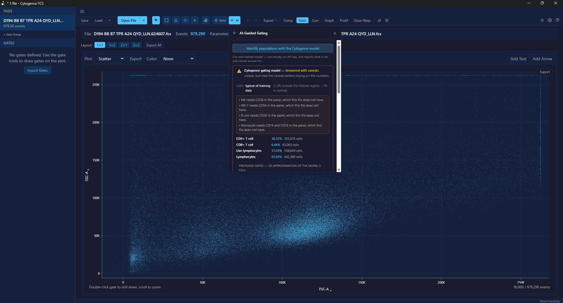
A real run on a T-cell panel. The novelty check passed — 1.2% of cells outside the trained region, where about 1% is normal — so the model is not abstaining because the data looks strange. It declines NK and NK-T for want of CD56, B cells for CD20, and monocytes for CD14 and CD16, naming each one. The four populations it can identify are reported underneath.

Those percentages are of all events

Every figure in the results card is a percentage of all events in the file — not of its parent population. In the run above, Live lymphocytes reads 57.05%: that is 57% of the whole file, and about 86% of the Lymphocytes gate it sits under.

The card heads them The model’s own call — per cell, % of all events, and hovering a figure says the same. The statistics table shows both denominators, with separate % Total and % Parent columns, so use it whenever the distinction matters.

These per-cell calls tell you how well the model fits the file. The figures to report come from the gates once you have reviewed and applied them — those are computed from the gate geometry, not from the model.

The proposed gates go to the gate list, one step at a time

When the model answers for any population, the card says how many steps it proposes — “5 steps proposed — review them in the gate list” — and the steps appear above your gate tree under Proposed — not yet gates.

The proposal is a hierarchy, not a flat set — scatter cleanup, then CD3, then CD4 and CD8 beneath it, for example. Nothing has been created yet and nothing is counted in your statistics. Each step names the parent it is waiting on, and you decide one step at a time:

• Apply creates that gate. A step needs its parent applied first.
• Revise changes how strict that cut is, and re-fits every step below it.
• Skip drops the step, and the steps waiting on it with it; Undo skip brings them back.
• Preview puts the plot on the step’s axes and shows its cut.

A scatter-cleanup step has no boundary for the model to propose: it asks you to Draw it on the plot, or to use a gate you already drew on those axes.

Strictness — Widest, Inclusive, Balanced or Strict — applies to every step not yet accepted. Stricter keeps only the cells the model is most sure of, at every step, so it finds a purer population and a smaller one.

Each step is an approximation, and it says so

The model’s decision uses every marker at once, which cannot be drawn as a shape on a 2D plot. So each step is a 2D gate that approximates the model’s call, and it shows how good that approximation is: “96% captured” means that of the cells the model selected, 96% fall inside the gate; “5% extra” means that of the cells inside it, 5% were not selected by the model.

That second number is the one to read. A gate with a lot of “extra” is a shape that happens to enclose cells the model rejected, so the drawn gate is looser than the model’s actual call.

Note that CD3 appears as a step even though it is not one of the reported populations — it is the stage the CD4 and CD8 chains pass through.

It checks compensation before applying

The model always reads each file with that file’s own acquisition compensation, whatever the workspace currently shows. If you have turned compensation off for the file or given it a different matrix, applying a step asks first — Compensation for AI-1 gates — and offers Use acquisition compensation and apply, because the same gate would otherwise count a different population. See Compensation.

Getting the best out of it

Name your channels. AI-1 identifies channels by the marker they measure, not by fluorochrome, detector or channel order — that is what lets it read panels it was never trained on. But it can only do that if the marker is actually recorded. A channel called FL4-A with no marker name is invisible to it.

Fix names in the parameter editor before running it. See The interface.

Keep the acquisition compensation when you apply its gates. The model reads each file with the file’s own acquisition matrix, and its gates are fitted there. If you have changed a file’s compensation, the app asks before applying them (above).

Read the report before the gates. If a population was declined, the gates it did produce are still worth having — but you now know which parts of the tree are yours to draw.

What it is, technically

A marker-semantic set encoder: each cell is treated as an unordered set of (marker identity, intensity) pairs, read by a small permutation-invariant transformer, with a thin head per population. Because a marker’s representation is keyed on biological identity rather than channel position, the encoder can read panels it never trained on.

It is small — its encoder has about 323,000 parameters — and implemented directly in Rust: no ML runtime, no GPU requirement, nothing to install.

Trained on publicly available human immunology studies with published expert gating. Patent pending.

Improving it

This version of the app collects nothing about your gating; nothing leaves your machine. Learning from the gates people correct is how AI-1 is meant to improve, and any such collection is opt-in, never opt-out. See Licensing.

When to use the copilot instead

AI-1 is the right tool for the populations on its list. For anything else — an unusual panel, a population it does not cover, or a strategy you want reasoned about in words — use the copilot, which plans in plain language and hands you each step to approve.